Principles of Finite Element Analysis

In my time at UM, I also served as a Graduate Student Instructor for the Mechanical Engineering department’s introductory Finite Element Analysis class. I aim to give a very short, non-technical summary of how this analysis method works.

Introduction

Stress contour plot of an FEA analysis — Numerical results from FEA are often color-coded with contour plots to make reading them easier.

The Finite Element Method is often used to give approximate answers to complicated physical problems. It is commonly applied to problems of mechanical, fluid, thermal and electromagnetic behavior.

Enabling Assumptions

At its heart are two assertions that drive its use:

We can answer simple questions easily. The invention of calculus has led physicists to develop models of physical behavior that are quite accurate to real-life for simple problems. Examples of this include the bending of a diving board as someone jumps on it, how heat conducts itself away from your hand into a cold metal railing you grasp, or how water flowing slowly in a river behaves.
Any complicated problem can be decomposed into a series of smaller, simpler subproblems, and the solution to the complicated problem can be reconstituted by summing up the solutions of these smaller, simpler subproblems.

The area under a graph is the sum of infinitely many small rectangles — Pardon the math, just focus on the visual idea of representing the area under a curve as the sum of thin rectangles of height equal to the curve at that point.

For those who recall or have taken some introductory calculus, this approach to problem solving is analogous to the approach taken with computing integrals: take any function and chop the area under its graph into a series of small rectangles and add up the areas of the small rectangles. The key difference is that the Finite Element Method uses a finite number of smaller terms, whereas integration uses limits to sum an infinite number of smaller terms. What makes FEA work is that after a certain number of smaller terms, the results don't change meaningfully. We call this convergence.

Finite Element Analysis for a physical deformation problem looks something like this: \(u = \sum_{n=1}^N \epsilon_n\) where \(u\) is the overall deformation of the part and \(N\) is some arbitrarily large number of smaller elements, and \(\epsilon_n\) is some mathematical expression that describes the material behavior, e.g. for linear elasticity, \(\epsilon_n = \frac{\sigma}{E}\) where E is the Young's Modulus of the material, a material parameter, and \(\sigma\) is the stress it is subject to, for element \(n\).

Application to FEA

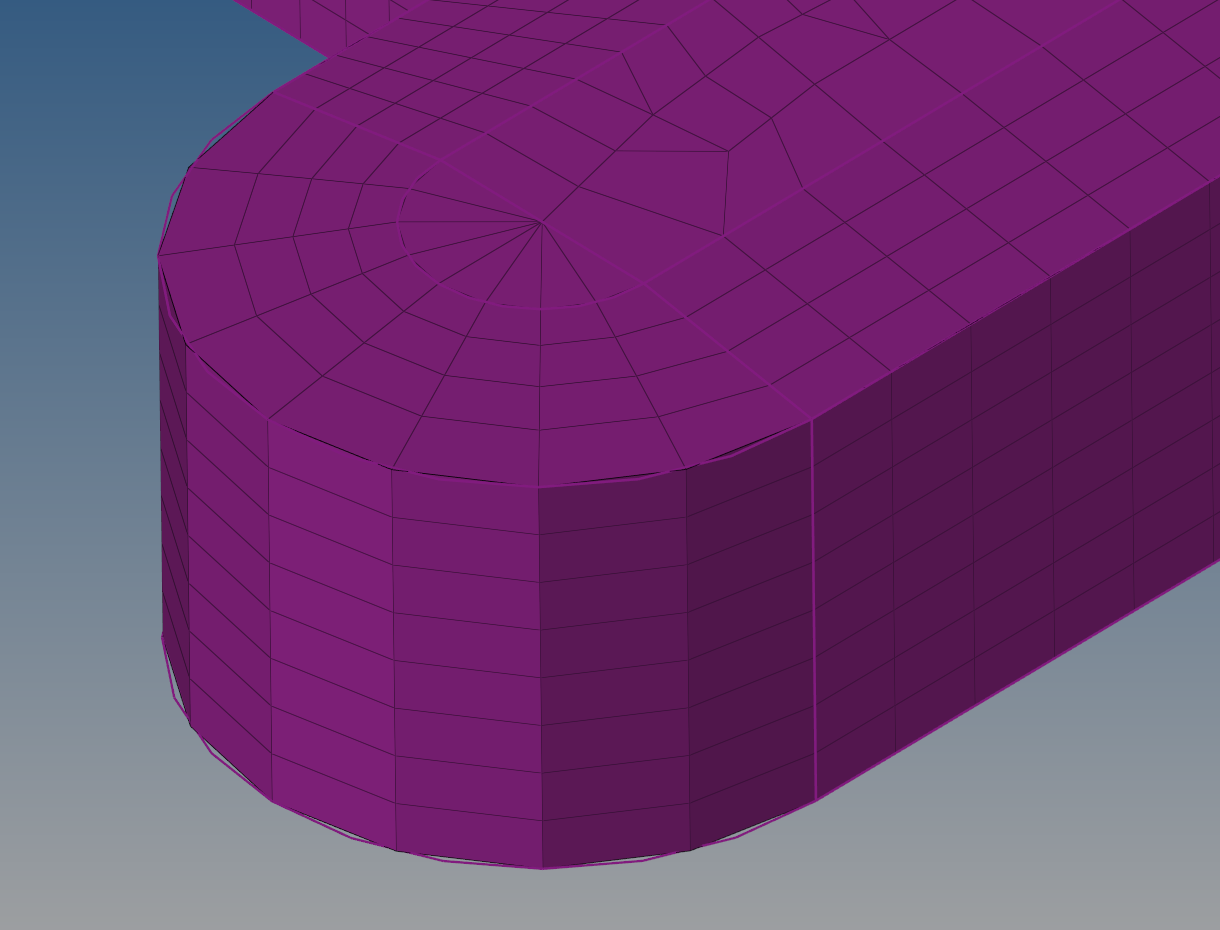
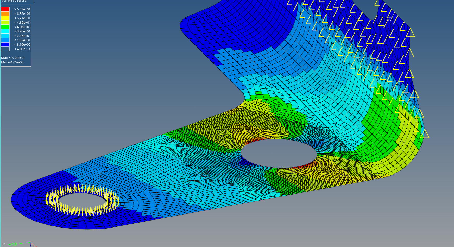
A smooth half-circle is replaced by a set of straight-edged triangles — FEA practitioners also have to make sure they use enough elements to approximate the geometry of their model well — use too few elements and a circle gets discretized into a square!

How this strategy manifests itself in Finite Element Analysis is primarily in how to chop up a complicated problem into smaller, simpler problems. We know how simple shapes like triangles, squares, tetrahedra and cubes behave, so we can chop any complicated shape up into a mesh of interconnected elements. Once we apply some known things about the analysis problem, e.g. how much force we are applying to a model, where the force is applied, and what material the model is made of, we can start from these boundary conditions and solve the physics problem we are interested in step by step until we have results for the entire mesh. Then, we can add these results up to approximate the behavior of the whole model!

Practical Considerations

The time it takes to solve FEA problems scales non-linearly with the number of elements. — When using supercomputers to solve problems, time is quite literally money!

Of course, the finer you chop up a problem, the more simple problems you need to solve. The rise of faster, more powerful computers has sped up the time it takes to solve these simple problems, so we can afford to make our meshes finer and finer, and include even more complicated physical models for each little element. However, at the end of the day, we have to decide on the number of elements we want and stick with that. This is where the “Finite” in Finite Element Method comes in. Of course, as we increase the number of elements, our results become more and more accurate, but at some point, we hit diminishing returns, where the time it takes to solve a problem outweighs the gain in accuracy. It is up to the skilled practitioner to decide when the tradeoff between time and accuracy is justified, and when to stop refining the model.

I hope this has given you some insight into how the Finite Element Method works!